This data repository holds the data for the Brake-Reuss Beam (BRB) measured in Dec, 2021. The repository contains:

Interface scan data captured using a Keyence VR-5100 white light interferometer,
Hammer Impact Tests
Shaker tests (random and sine forcing) with an array of sensors

The first section provides some details about the experiments, but more details on the data can be found in the following publications:

Balaji, Nidish. "Dissipative dynamics of bolted joints." PhD diss., Rice University, 2021. (link)
"Influence of Wear on the Nonlinear Dynamics of a Lap Joint Structure: Observations from Long-Term Experimentation", Balaji, N. N., Smith, S. A., and Brake, M. R. W. (Under Preparation)

The dataset can be accessed here, through OSF. The following is the citation information of the dataset

Balaji, Nidish N, Matthew Brake, and Scott A Smith. 2023. “BRB_LTERM_MULTISCALE21.” OSF. December 18. doi:10.17605/OSF.IO/GHKJ7

Contact Details:

Nidish Narayanaa Balaji: nidish.balaji@ila.uni-suttgart.de
Scott A. Smith: ssmith18@norwich.edu
Matthew R. W. Brake: brake@rice.edu

Experimental Details

Overview

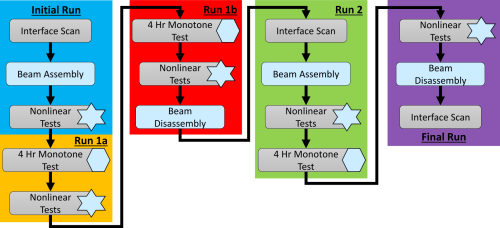
The data were collected over a 12 hour experimental campaign conducted in this sequence:

Interfaces were scanned initially
Beams were assembled and impact tests were conducted
Step sine and Random tests were conducted with the shaker
A single sine excitation was provided to the assembly at 172Hz for 4 hrs
Step Sine and Random tests were conducted with the shaker
A single sine excitation was provided to the assembly at 172Hz for another 4 hrs
Step Sine and Random tests were conducted with the shaker
The beams were **disassembled** and the interfaces were scanned after cleaning
The beams were assembled again and step sine and random tests were conducted
A single sine excitation was provided to the assembly at 172Hz for a final 4 hrs
Step sine and Random tests were conducted with the shaker
Hammer impact tests were conducted
The beams were **disassembled** and the interfaces were scanned after cleaning

Sensor Configuration

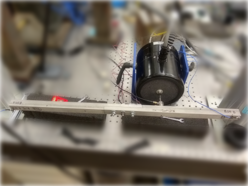
For all the shaker tests, the following 15 channels can be found

Excitation Force (N)
Strain Gauge 1 (eps)
Straing Gauge 2 (eps)
Straing Gauge 3 (eps)
Acceleration at Excitation Point (g)
X Accel, left end in figure (g)
Y Accel, left end in figure (g)
Z Accel, left end in figure (g)
X Accel, right end in figure (g)
Y Accel, right end in figure (g)
Z Accel, right end in figure (g)
Thermocouple 1 (deg C)
Thermocouple 2 (deg C)
Thermocouple 3 (deg C)

Interfacial Scan Data

Six datasets are provided:
`R05A_Before`

Interface "A" before any testing (mint-condition)

`R05B_Before`

Interface "B" before any testing (mint-condition)

`R05A_After`

Interface "A" after the first round of 8hr testing

`R05B_After`

Interface "B" after the first round of (8hr) testing

`R05A_After2`

Interface "A" after the second round of (4hr) testing

`R05B_After2`

Interface "B" after the second round of (4hr) testing

For each dataset, the height data are provided in a csv file named as: `<date>_<beam_identifier>_S<index>_<misc>.csv`
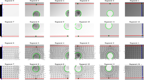
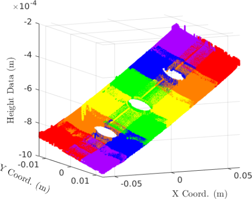
- Here, the `S<index>` portion indicates the "Segment Index" going from 1 through 12, since the whole interface
The relevant scripts are,
- `scan_a_rawdat2meshsort.m`
- `scan_b_visdata.m`
- `scan_c_elemaspID.m`
The first script, `scan_a_rawdat2meshsort.m`,
- Loads the raw data
- Loads a finite element mesh
- Processes the raw data (outlier rejection, patch-joining, etc.)
- Sorts the data into different elements, and
- saves it into a mat-file.
The second script, `scan_b_visdata.m`,
- Loads the processed data from the first script (you have to run the first script first)
- Makes basic plots, demonstrating the use of the data
The third script, `scan_c_elemaspID.m`,
- Loads the processed data from the first script (you have to run the first script first)
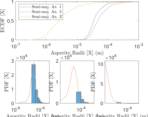
- Shows how to extract statistical properties of the asperities
Here are samples of the data through the processing steps:

Hammer Impact Test Data

Two sets of impact test data are provided, labeled "Initial" and "Final"
The "Initial" data corresponds to the impact tests conducted right after assembling the beams for the first time
The "Final data corresponds to the impact tests conducted after the 12 hour experimental campaign concluded
The data can be found in the `DATA/IMPACT_DATA/` folder
A MATLAB script `impact_a_loadshow.m` shows how to load and plot the data

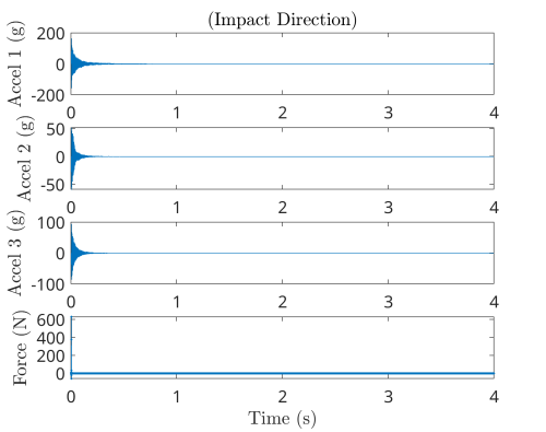
The first channel in `Signal_1` is the acceleration along the direction of input

Shaker Test Data

3 sets of shaker test data are provided,
- `FirstRound_16Dec2020` : The first round. Includes
  `RandFRF_Before`, `RandFRF_After`
  
  Random FRF Test
  
  `StepSine_Before`, `StepSine_After`
  
  Step Sine Tests
  
  `SingFreqTest`
  
  Single Frequency Test
- `SecondRound_17Dec2020` : The second round. Includes
  `RandFRF_After`
  
  Random FRF Test
  
  `StepSine_After`
  
  Step Sine Test
  
  `SingFreqTest`
  
  Single Frequency Test
- `ThirdRound_18Dec2020` : The final round. Includes
  `RandFRF_Before`, `RandFRF_After`
  
  Random FRF Test
  
  `StepSine_Before`, `StepSine_After`
  
  Step Sine Tests
  
  `SingFreqTest`
  
  Single Frequency Test
All the shaker data are collected in the time domain so the postprocessing scripts provided below also do the time-to frequency domain conversion

Single Frequency Tests

Three sets corresponding to the three 4 hour tests are provided,
- `FirstRound`
- `SecondRound`
- `ThirdRound`
The data are provided as CSV files with names following the convention: `<prefix>_V<vlevel>_singfreq<index>.csv`
For example, the file `FirstRun_V1.2_singfreq100.csv` specifies the data from the `FirstRun`, undergoing an excitation of `1.2 V` at the stated frequency (172 Hz everywhere).
- The index 100 implies that this is the 100th file recorded for this case.
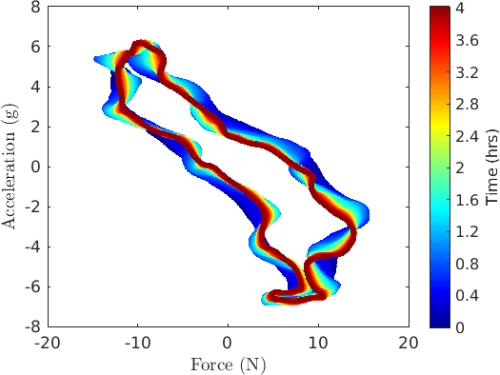
- Each file is a block recorded once every \~140seconds (the exact value can be obtained from `(Testinfo.SaveBlocks+Testinfo.IntervalBlocks)*Tblock` in the code).
- The file with `<index>` 0 corresponds to test conducted with zero inputs (this can be used to estimate noise)
The rows are organized as follows:
Row 1

Name of channel

Row 2

Sampling time Δ t (s) of channel (each channel can be sampled differently based on the type of sensore: ICP, strain gauge, thermocouple, etc.)

Rows 3-

The data corresponding to each channel
The MATLAB Script `singfreq_a_postproc.m` shows how these are postprocessed and written into .mat files
The MATLAB Script `singfreq_b_makeplots.m` shows how to load the .mat files produced by the first script to make plots

Random FRF Test

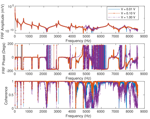
Five sets of random FRF data are provided,
`FirstRound/RandFRF_Before`

The tests done

`FirstRound/RandFRF_After`

Done after 4hrs of monotone tests

`SecondRound/RandFRF_After`

Done after 8 hrs of monotone tests

`ThirdRound/RandFRF_Before`

Done after reassembly

`ThirdRound/RandFRF_After`

Done finally

The data files are provided as csv files with naming convention:

   <prefix>_V<level>_randfrf<index>.csv

where `<prefix>` & `<level>` mean the same as before, but `<index>` implies the realization of the random excitation test.

For example, the file `FirstRun_V1.0_randfrf9.csv` implies that it was the 9th repeat collected as part of the `FirstRun`, with an RMS input voltage of `1.0 V`
The data are provided as csv files with rows organized similar to above, as
Row 1

Name of channel

Row 2

Sampling time Δ t (s) of channel (each channel can be sampled differently based on the type of sensore: ICP, strain gauge, thermocouple, etc.)

Rows 3-

The data corresponding to each channel

The script `randfrf_a_postprof.m` provides MATLAB code to load and postprocess the data appropriately
The script `randfrf_b_plots.m` shows how to load the data from the above to plot the FRF

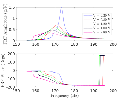
Step Sine Tests

"Open-loop" Step-sine tests were conducted by imposing different voltage amplitudes and stepping through a set of frequencies
Similar to before, five sets of step sine test data are provided.
`FirstRound/StepSine_Before`

First set of step sine

`FirstRound/StepSine_After`

Done after 4hrs of testing

`SecondRound/StepSine_After`

Done after 8hrs of testing

`ThirdRound/StepSine_Before`

Done after reassembly

`ThirdRound/StepSine_After`

Done after final 4hrs of testing

The time-domain data are provided in csv files named with the convention:

   <prefix>_V<level>_stepsine<index>.csv

where `<index>` corresponds to different frequency points along the step sine curve.

The rows of the data files are
Row 1

Channel name

Row 2

Channel sampling time Δ t (s)

Row 3

Excitation frequency (Hz)

Rows 4-

Recorded data for each channel

The script `stepsine_a_postproc.m` shows a sample of the postprocessing done in MATLAB
The script `stepsine_b_makeplots` shows how to make plots using the data.

Data Access Details

The data has been uploaded to OSF and can be freely accessed here.
Apart from the data, MATLAB scripts have been provided to make the access easy.
The subdirectories in DATA/SHAKER_DATA/ contain zip files which must be unzipped first, upon download, so the matlab scripts can work.
The total data set is approximately 10GB.
If you use this data in your work, please consider citing,
1. Balaji, N. N. "Dissipative dynamics of bolted joints." PhD diss., Rice University, 2021. (link)
2. Balaji, Nidish N, Matthew Brake, and Scott A Smith. 2023. “BRB_LTERM_MULTISCALE21.” OSF. December 18. doi:10.17605/OSF.IO/FBWHZ.
3. Balaji, N. N., Smith, S. A., and Brake, M. R. W. "Influence of Wear on the Nonlinear Dynamics of a Lap Joint Structure: Observations from Long-Term Experimentation" (Under Preparation)

Multi-Scale Data from Long Term Vibration Tests Conducted on The Brake-Reuss Beam (2020-21)

Contents